
1.The select distinct Statement
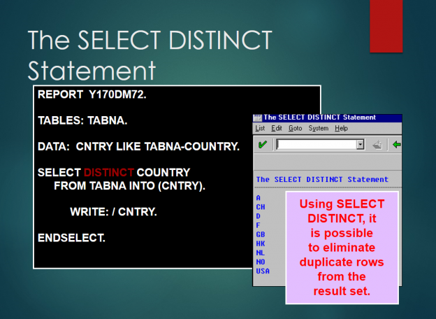
•The SELECT DISTINCT option is used to return only one record for each unique occurrence of data in a column based on a field name (or combination of field names). All other records that have the same matching data, will not be included in the result set.
•It is recommended you use very few columns with the SELECT DISTINCT option. The result tends to lose significance if too many columns are specified.
•The SELECT DISTINCT requires an INTO clause because it is selecting
individual columns.
individual columns.
Performance Tips:
When handling large amounts of data (>10 MB) and selecting with the support of an index, SELECT DISTINCT is the most efficient syntax (to check for index support, use transaction ST05 – see help on SQL Trace Tool). However, if the amount of data is small and there is no index, fill an internal table and then use the DELETE ADJACENT DUPLICATES statement.
2.SELECT Using Aggregate Functions
• The aggregate functions MIN, MAX, AVG, SUM, and COUNT are a valuable tool for accumulating values across the entire table or a subset of the table rows based on the conditions in the WHERE clause.
• Notice there is no ENDSELECT because the aggregate SELECT statement does not return multiple records.
• Aggregate functions require an INTO clause because they return single values.
• After the aggregate name, you must specify the individual columns of interest within parenthesis.
• The open (left) parentheses must come immediately after the aggregate function – no space is allowed here.
• The field name inside the parenthesis must be preceded by a space and followed by a space (before and after the open and close parenthesis).
• When using DISTINCT in an aggregate expression, the aggregate function does not apply to all of the values in the table. The function only applies to those different or DISTINCT values. In the case above, the COUNT aggregate function is applied to only those distinct nine countries not to the entire table.
• Aggregate functions cannot be used with pooled or cluster tables.

• Performance Tips:
• Aggregate functions are executed at the database level and, therefore, increase efficiency -this is further enhanced by the use of the GROUP BY statement.
3.The Dynamic WHERE Clause
•The WHERE clause is created at runtime and can be created by the user
using parameters.
using parameters.
•An internal table must be created which can only have one field. The field must be type C and should not exceed 72 characters.
•The following restrictions apply to the conditions:
–Only literals can be used as values, not variables.
–The IN operator cannot be used in conjunction with the internal table
[as in <field1> IN (itab) ].
[as in <field1> IN (itab) ].
•The where clause internal table can be empty. In this case the SELECT statement will be executed as if there was no WHERE clause (all rows returned).
•It is possible to specify an additional condition within the WHERE clause outside the internal table. The syntax is as follows:
–WHERE <condition> AND (itab)

4.CONCATENATE Statement
•CONCATENATE is a string processing statement which enables the programmer to combine the contents of one or more source fields into a single target field.
•After the CONCATENATE statement is executed, the SY-SUBRC system field will contain one of the following values:
•0 – the source field fits successfully into the target field
•4 – the source field is too big for the target field and was truncated to the size of the target field
•The option SEPARATED BY is useful for embedding spaces or special characters between the multiple source fields before they are transported to the target field.
•In the example above, the CONCATENATE statement is used to construct a WHERE clause in a SELECT statement. The user enters the various options and/or conditions that make up the WHERE clause on a parameter screen. The program takes the parameters and CONCATENATES them into a comprehensive WHERE clauses separating each condition and operator with a space.

5.Variation on the INTO Clause
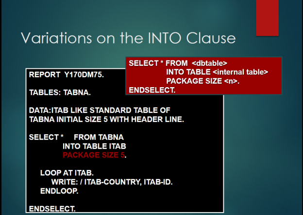
• Reading selected rows into an internal table in packages of a predefined size is possible using the PACKAGE SIZE <n> option with the INTO clause.
• The SELECT statement with the PACKAGE SIZE option initiates a loop which is terminated with an ENDSELECT statement. For every package of <n> rows the system makes one pass through the loop.
• Outside the SELECT loop, the contents of the internal table are unknown. Therefore, any processing on the rows that is to be performed, must be done inside the SELECT … ENDSELECT loop.
• In the example above, all rows of TABNA are read into TAB in packages of 5 rows. Inside the SELECT loop a second loop is nested in which the packages are written to the report.
• Performance Tips:
• The INTO TABLE statement can be used without the package size addition. This is a more efficient code than a SELECT …. ENDSELECT, as the database access is reduced – all records meeting the selection criteria are moved into the table in one process, so no database looping is required. The internal table can then be looped at for further processing.
6.Specifying the Table Name at Runtime
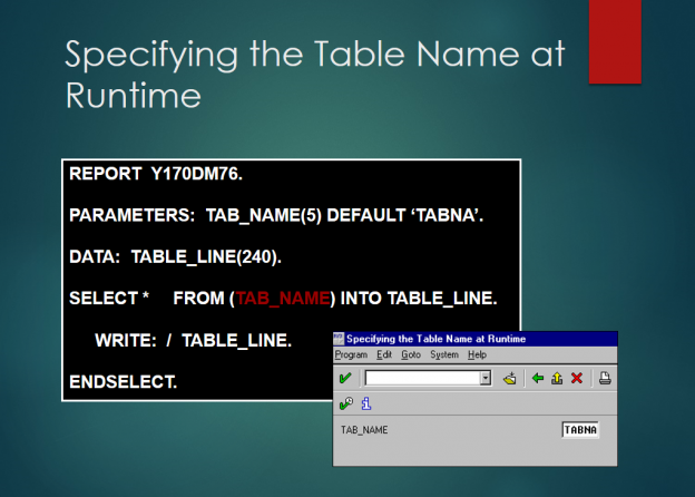
• Using dynamic table specification, it is possible to designate the name of the
table to select records from at run time.
table to select records from at run time.
◦ In the example above, the table name is passed to the program through a parameter and then used in a SELECT statement.
• Notice there is no TABLES statement. Specifying the table name at runtime is the only time in Open SQL that a TABLES statement is not needed to declare the table work area.
• In this form, it is required that the data be read into a work area or internal table.
◦ Since the name of the table is not known until runtime, it is necessary to make sure the work area is large enough to accommodate the length of the records it will be holding.
• Since the generation of internal control blocks occurs only at runtime, a SELECT statement with a dynamic name specification impairs performance more than a static name specification.
• It is possible to use the ORDER BY PRIMARY KEY, but not ORDER BY f1.
7.Joins: Why We Should Use Them
•Previously, in order to access multiple tables, we used nested selects either directly coded into our program or through a logical databases. Both of these methods have drawbacks:
–Nested selects cause a significant amount of overhead when accessing the database. For instance, a select statement, nested within a select loop, would have to be executed with each record the outer select statement retrieves. Not only does this increase network traffic, but each time a select is executed, process control is shifted between the DBMS and your ABAP program. These process control shifts take time, consequently, causing inefficiency.
–Logical databases, although useful and easy to code, are also inefficient due to the nested selects they use. In fact, logical databases are more inefficient than ordinary nested selects, do to additional process control shifts between the primary ABAP program, and the logical database program.
•Joins have the advantage of accessing multiple tables with one Select statement, thereby reducing the amount of server overhead.
•Joins will always bypass the buffer.
Inner joins are new as of 3.1h, and left outer joins are new as of 4.x.
8.Inner Joins
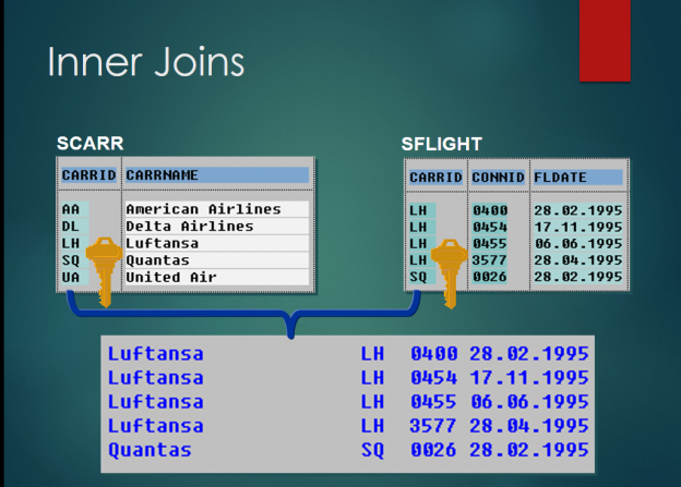
• Inner Joins allow access to multiple tables with a single select statement by creating a temporary table based on the conditions in the ON statement. Inner Joins are equivalent to views created in the Dictionary (see appendix – Data Dictionary).
• Aside: In all slides in this chapter, illustrations of scarr, sflight and sbook contain all records for the fields displayed.
• Syntax for inner join above:
• SELECT scarr~carrname sflight~carrid sflight~connid sflight~fldate
• INTO (carrname, carrid, connid, date)
• FROM scarr INNER JOIN sflight
• ON scarr~carrid = sflight~carrid.
• WRITE: / carrname, carrid, connid, date.
• ENDSELECT.
• Multiple tables are joined based on key fields specified by the join condition. The output list displayed above is the result of an inner join on the CARRID field of the SCARR and SFLIGHT tables. The result of an inner join will be identical, regardless of whether the condition is expressed in an ON or WHERE clause.
9.Inner Joins Syntax
•In order to access multiple tables, we must specify the table name of key fields that are found in both tables in the field list.
•E.g., SELECT sflight~carrid sflight~connid fldate carrname
–fldate and carrnam do not need to be prefixed with there respective Database table name, because each only exist in one of the two accessed tables.
–However, you should consider prefixing all fields with their respective table names, for the sake of clarity, and to allay any conflicts if identical fields are added to one of the joined tables in later versions of SAP.
E.g., SELECT sflight~carrid sflight~connid sflight~fldate scarr~carrname
•You can specify multiple table fields in the ON clause as seen in the slide above.
•“Inner join” can be replaced with just “join”.

10.The Driving Table
• The table hierarchically higher in an inner join should be the driving table (A.K.A., The Left-Hand table). In the slide above, theoretically scarr would be hierarchically higher than sflight in the FROM clause, since it deals with specific flight information. Scarr deals with the airline names associated with the carrid field.
◦ Tables lower down in the hierarchy are usually larger and more specific than those higher.
◦ This can also be seen when using nested selects. The code below will produce output identical to the code on the slide above.
• SELECT carrid carrname FROM scarr
• INTO (scarr-carrid, scarr-carrname).
• SELECT carrid connid fldate FROM sflight
• INTO (sflight-carrid, sflight-connid, sflight-fldate)
• WHERE carrid = scarr-carrid.
• WRITE: / scarr-carrname, scarr-carrid,
· sflight-connid, sflight-fldate.
◦ ENDSELECT.
• ENDSELECT.
· Here and in the slide above, the driving table is scarr (it is just coincidence that the “driving table” is named scarr ).

11.The Left Outer Joins
• Like inner joins, left outer joins create a temporary table based on the conditions specified in the ON clause.
• Unlike inner joins:
◦ Based on conditions expressed in the ON statement, fields in the driving (left-hand) table that do not correspond to fields in the right-hand table are still added to temporary table. There they are populated with initial values.
◦ The non-corresponding records’ fields in the right-hand table are populated with initial values in the resulting temporary table, thus producing the output displayed above.
◦ However, this is not the case with the WHERE condition – records not found in both tables are eliminated.

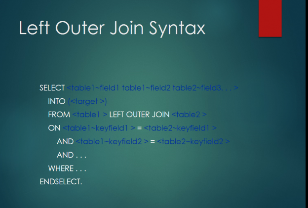
12. The Left Outer Joins Syntax
• Aside from the FROM clause, the syntaxes for inner and outer joins are identical.
◦ The “OUTER” in “LEFT OUTER JOIN” can be omitted.
• Outer joins have syntax restrictions additional to those shared with inner joins (see next slide).
◦ Conditions in the on clause can only be “=.“
· E.g., no “sflight~carrid < spfli~carrid.”
◦ The ON condition must contain a field from the rightmost table.
◦ The WHERE condition can only contain fields from the leftmost table.
13.Open SQL Syntax Restrictions
• Not all databases supported by SAP share a standard syntax for the ON clause. This means that the results of a join may differ depending upon which database is being used. Because of this, the syntax for joins have been given certain restrictions in order to insure that they produce the same results for all SAP supported databases:
• Only a table can come after the JOIN statement.
• I.e., “From SFLIGHT left join SBOOK left join SPFLI” would give you a syntax error.
• Only the AND logical operator can be used in the join condition.
• Each comparison in the ON condition must have a field from the right hand table.
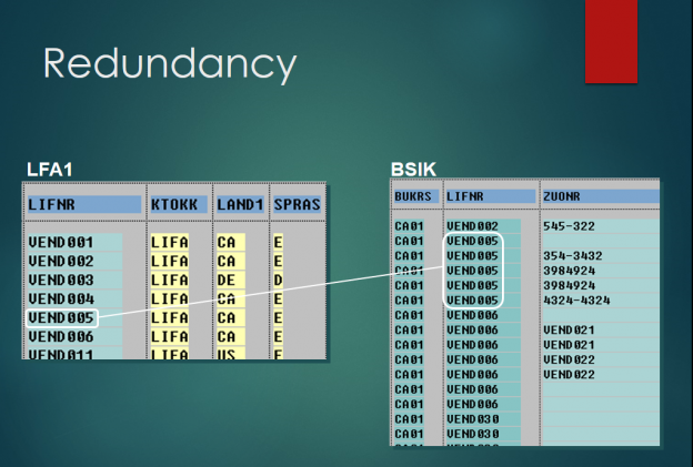
14.Redundancy
• Joins have the disadvantage of returning redundant data when the left and right tables have a 1:N relationship. I.e., for every record in the driving table, there may exist multiple records in the right hand table. For instance, a vendor in the LFA1 table may have many documents associated with it in the BSIK table.
• Because of this redundant data, the amount of data being passed between the database layer and the application layer is quite large. For this reason, you should only select fields that are absolutely necessary.
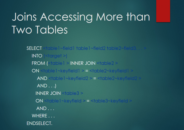
15.Joins Accessing More than Two Tables
•In order to join multiple tables, you must: first join two tables, put them into parentheses, and then join the next table (on slide above).
–To join more than three tables, you would put the first three tables in parentheses, and then join the next table.
E.g., ((tab1 INNER JOIN tab2 ON…) INNER JOIN tab3 ON. . .) inner join tab4 ON. . .
–Generally, you will not join more than three tables.
–The syntax for outer joining more than two tables is the same.
16.Aliases
• Aliases simply allow the programmer to prefix fields with shorter table names. This comes in useful with long field lists.
• You can only use a table alias to prefix a database field not a work area (I.e., a tilde (~) must follow the alias). E.g., A-carrname would be incorrect.
• Aliases have no impact on performance.

17.Subquery
•Subqueries are a more efficient method of performing complex select statements.
•The conventional method of coding a solution to the question posed in the slide above is:
SELECT * FROM scarr.
SELECT * FROM sflight WHERE carrid = scarr-carrid.
ENDSELECT.
IF sy-subrc >< 0.
WRITE:/ scarr-carrid, scarr-carrname.
ENDIF.
ENDSELECT.
–Because of the nested select and the comparison of the scarr-carrid work area with the sflight~carrid database table field, there is an excessive amount of data being transferred between the application and database layer. I.e., All data from both select statements is being sent to the application where it is then processed (in this case, by IF SY-SUBRC).
–Subqueries can handle this at the database layer; therefore, the data that has to be transferred to your program is reduced. In the case of the slide above, only three records would have to be transferred back to the application.
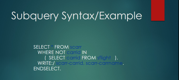
18.Subquery Syntax/Example
• The code in the slide above will produce identical output to the code in the previous slide.
• You cannot use SELECT SINGLE with subqueries.
• Some other conditions in the where statement include:
◦ WHERE <field>IN
◦ WHERE EXISTS ( SELECT. . .
· This can be used in a select statement that will produce one record.
◦ WHERE NOT EXISTS ( SELECT. . .
· In both EXISTS and NOT EXISTS the subquery (I.e., the select in parentheses) is executed last.
· Aside: You can alias the table name with:
◦ Select * FROM scarr as A WHERE. . .
19.Having Clause
•The having clause assigns the selection criteria handling to the database instead of the application server. Similar to the subquery, the advantage of this is the reduction in the amount of data being transferred between the two layers.
•The conventional method of coding a solution to the query in the slide above would be:
SELECT carrid connid COUNT(*) SUM( luggweight )
INTO (carrid, connid, count, sum_weight)
FROM sbook
WHERE carrid = ‘LH’
GROUP BY carrid connid.
IF sum_weight > 25.
WRITE:/ carrid, connid, count, sum_weight.
ENDIF.
ENDSELECT.
–Since we are using an IF statement at the application server level to process the selection criteria, every record that satisfies the WHERE condition is transferred to the application. However, in the case of the HAVING clause, only the records that satisfy the WHERE clause and HAVING clause are returned to the application, thus reducing the amount of data being passed back and forth.

20.Having Clause Syntax/Example
• The code on this slide will produce identical output to the code on the previous slide.
• HAVING must be used with aggregate expressions.
◦ Any fields in the field list not using aggregate expressions must be in the GROUP BY clause.
